Implementing a regression discontinuity design in R
1. What is the regression discontinuity design?
Chasing causality: Randomized controlled trials
Suppose we are interested in the causal effect a certain treatment has on certain properties, for example the causal effect a certain drug has on the resting pulse. The idea to get to the causal effect is simple
- Choose two groups and check the properties (in our case we would measure the resting pulse) we are interested in.
- Give the treatment (in our case the drug of interest) to one of the groups.
- Check the properties of interest again. The differences between the two groups are interpreted as the causal effect of the treatment.
Problem: That differences between the groups are causal effects of the treatment is only plausible if the groups are equal in all relevant properties except for the receivement of treatment. If they are not, differences after the treatment could also be due to differences before the treatment.
Solution: The solution is randomization. If we take random samples from the same population, they have the same expected value. According to the law of large numbers two random samples of the same population are therefore basically equal if the sample size becomes large enough. So randomization is a way to eliminate the problematic differences between the treatment and non-treatment group. To get back to our example: If we have a large enough group of people and randomly assign them to two groups, the expected mean resting pulse will be equal among the groups. But not only the resting pulse but also all other properties that might have an influence on the resting pulse, even those that we can’t control for. Since randomization rules out differences between the groups as possible causes of differences after the treatment, we can now interpret any remaining differences as causal effects of the treatment. This is what makes so-called randomized controlled trials (RCT) the gold standard for effectiveness research.
Problem: It is not always possible to conduct RCT. If we want to assess the effect of certain political measures for example it can be difficult to randomly assign whether someone gets the treatment or not. If we are interested in the effect of a certain tax for example, it would probably be quite problematic to randomly tax some people while others don’t have to pay the tax.
Regression discontinuity design
Regression discontinuity designs (RDD) are quasi-experimental designs that exploit cut-offs, for example in political measures, to form a control and treatment group that are - at least close around the cut-off date - equal without the need for randomization. To get back to our tax example. While people might protest if they are randomly chosen to pay a tax while others don’t have to pay, new taxes are introduced every now and then. Suppose that everyone has to pay a new tax from a certain date on. The idea of RDD is to form two groups: One before the cutoff date and one after the cutoff date. The necessary assumption for RDD to work is that both groups are equal except for having to pay the tax or not, at least shortly before and after the cut-off date. It is not implausible to assume that a population does not significantly change the moment a new tax is introduced. That assumption can be violated though, for example if a lot of political measures change around the same date. The question whether the two groups can be considered to be equal has to be judged case-by-case. If they can be considered equal though, we can treat the differences in the groups as causal effects again. So basically we exploit external cut-offs of some sort to create control and treatment groups and then treat them as we would treat them in a RCT, i.e. look at the differences between the groups after the treatment and interpret that difference as a causal effect of the treatment.
2. How to implement RDD in R
General idea
The general idea of implementing RDD in R is pretty easy: We apply a linear regression model and include a dummy variable indicating whether an observation is before or after the cut-off date. The effect of that dummy variable is than considered to be the causal effect of treatment. RDD are therefore implementation-wise basically just regular linear regressions, as we will see shortly.
Preparations
Loading necessary R packages.
library(rio)
library(AER)
library(lmtest)
library(sandwich)
library(stargazer)
library(modelsummary)
library(ggplot2)
Creating a function to plot the regression curves
The following function is used to create illustrations of the regressions.
plot_with_ci = function(model, response = anyrecid, lim_bandwith = F, lower, upper){
  # create predicted values of "model":
  model.pred = as.data.frame(predict(model, interval = 'confidence'))

  # create graph if bandwidth is not restricted:
  if (lim_bandwith == F) {
    ggplot(flo, aes(x=date, y={{response}}, group = after)) +
      # draw confidence intervals from predicted values:
      geom_ribbon(aes(ymin = model.pred$lwr, ymax = model.pred$upr), alpha = 0.5)+
      # draw regression line from predicted values:
      geom_line(mapping=aes(y=predict(model))) +
      # add model name as title
      ggtitle(deparse(substitute(model)))
  }

  else{

    # If bandwith is restricted: As above just with a subset and distnoab instead of date
        if (lim_bandwith == T) {
      flo_subset = subset(flo, distnoab >= lower & distnoab <= upper)

      ggplot(flo_subset, aes(x=distnoab, y={{response}}, group = after)) +
        geom_ribbon(aes(ymin = model.pred$lwr, ymax = model.pred$upr), alpha = 0.5)+
        geom_line(mapping=aes(y=predict(model))) +
        ggtitle(deparse(substitute(model)))
    }
  }
}
Importing data
Importing the data set “fl_offenders_ewifo.dta”:
flo <- import("fl_offenders_final_ewifo.dta")
The data is taken from Tuttle, C. (2019), Snapping Back: Food Stamp Bans and Criminal Recidivism, American Economic Journal: Economic Policy 11(2), S. 301-327’. Tuttle looks into the influence of foodstamp bans on recidivism. The cut-off that will be exploited and enables the use of the RDD is a change in the access to foodstamps. A change of law “suddenly” banned certain convicts from receiving foodstamps. For details see Tuttle’s paper. Tuttle applies the very same method that is presented here, so anything else than the actual implementation in R Tuttle’s paper is the right place to look.
The data set contains data on offenders, who committed drug offenses on or after the 01. October 1995 in Florida and were convicted.
Note: The data variables in the data set are measured as days since 01. January 1960.
Relevant variables
| Name | Description |
|---|---|
| date | Date the offense was committed (= ‘running variable’) |
| distnoab | Number of days since 23. August 1996 ( = ‘centred running variable’) |
| anyrecid | Dummy variable, =1 if person recidivated (all crimes), else 0 |
| finrecidany | Dummy variable, =1 if person recidivated (financially motivated crimes), else 0 |
| nonfinrecidany | Dummy variable, =1 if person recidivated (non-financially motivated crimes), else 0 |
| after | Dummy variable, =1 if date >= ‘1996-08-23’, else 0 |
2. Sharp RDD-Estimate
Sharp RDD are of such kind were there is a sharp cut-off date, i.e. before the cut-off date no-one received the treatment and after the cut-off date everyone received the treatment. The opposide is a fuzzy RDD, where getting the treatment becomes merely more likely when crossing the cut-off date. Since in our case a sharp cut-off date is given the fuzzy design won’t be considered here. As said before a sharp RDD is basically nothing more than a regular linear regression model with a dummy variable that indicates before/after the cut-off date. Using “anyrecid”, “after” and “date” the implementation in R is as simple as it gets:
rdd.1 <- lm(anyrecid ~ after + date, data = flo)
#summary(rdd.1)
plot_with_ci(rdd.1)
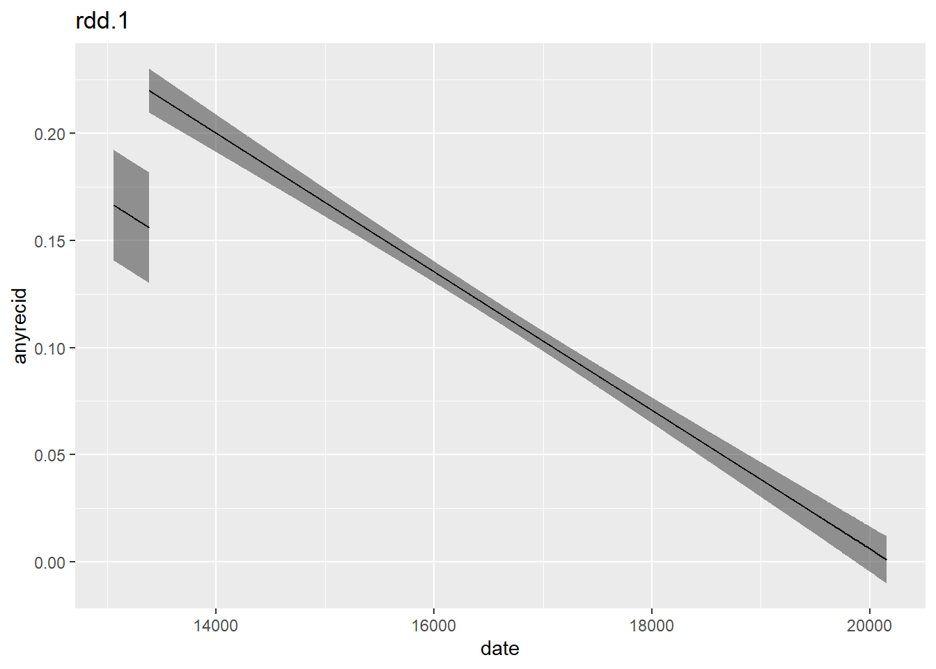
The figure illustrates the change around the cut-off date: After the cut-off there is an increase in recidivism. To get more informations on the model use the summary command that is included as a comment. The output is excluded here but we will soon look into it when comparing different models.
Is the increase in recidivism due to the change in legislature or is it actually a sign of a non-lineaer relationship between date and recidivism? After all, maybe the linear asssumption in our model is mistaken. To test this we can include a quadratic term for date.
rdd.2 <- lm(anyrecid ~ after + date + I(date^2), data = flo)
plot_with_ci(rdd.2)
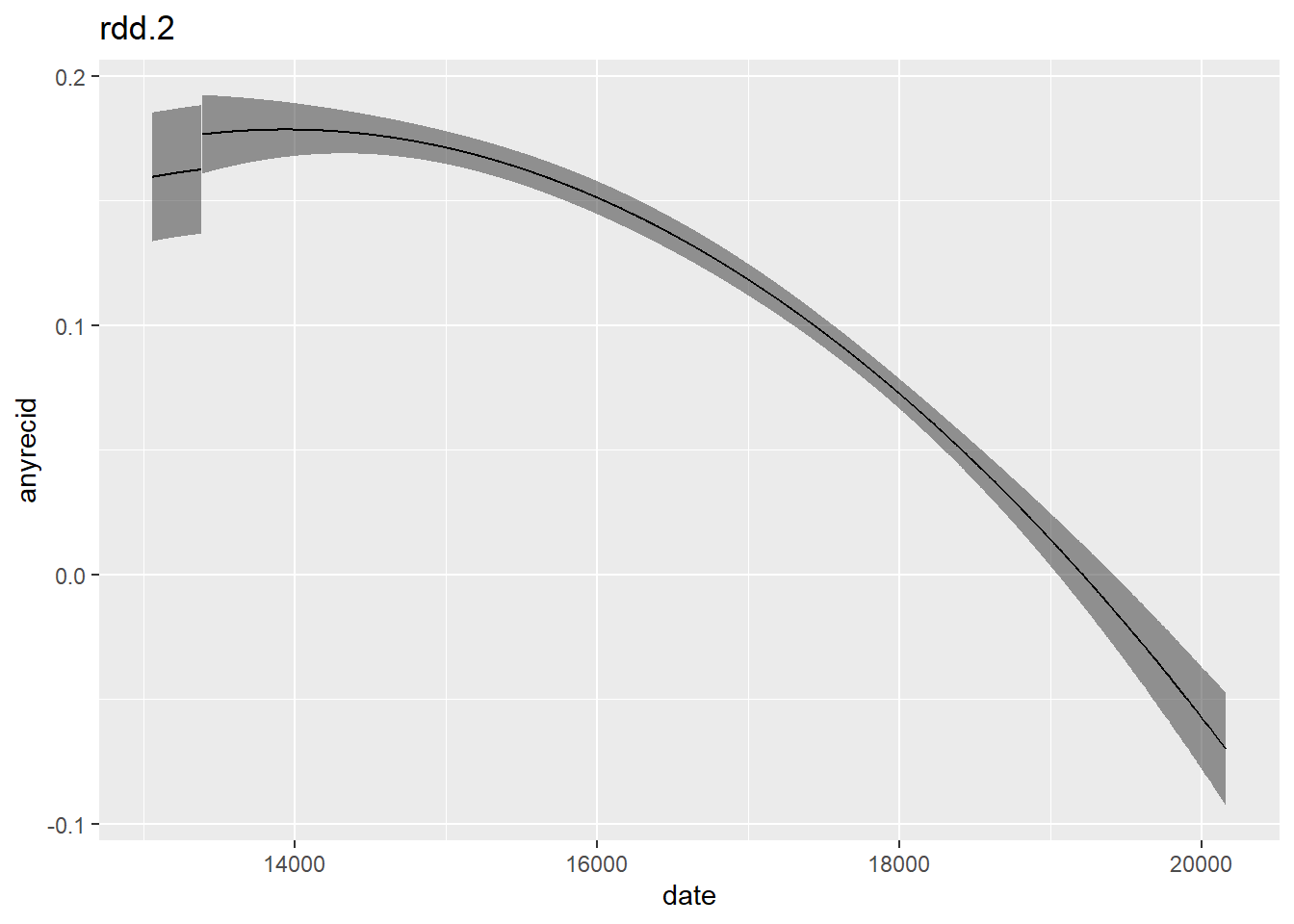
The quadratic model suggests that there is no statistically significant effect of the change in legislature but simply a non-lineaer relationship between date and recidivism
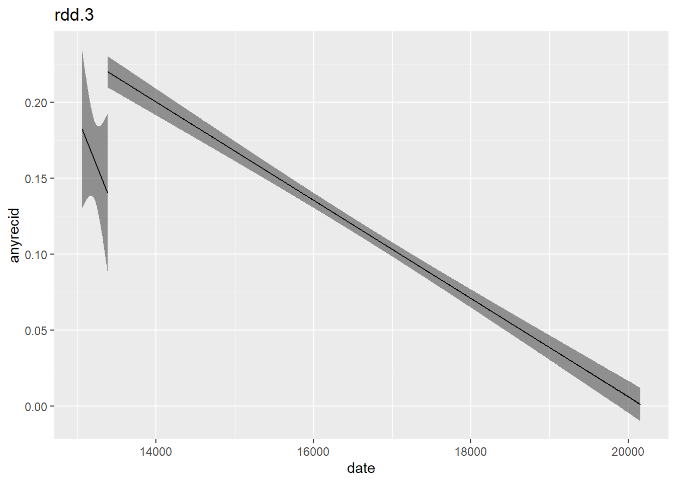
Another modification of the simple model is using the centred running variable distnoab with an interaction term. Doing so allows different slopes before and after the cut-off:
rdd.3 <- lm(anyrecid ~ after * distnoab, data = flo )
plot_with_ci(rdd.3)
Comparing models using the modelsummary package:
models = list(
"rdd.1 'Basic'"  = rdd.1,
"rdd.2 'Quadratic'"  = rdd.2,
"rdd.3 'Interaction'"  = rdd.3
)
modelsummary(models,
             stars = TRUE)
| rdd.1 'Basic' | rdd.2 'Quadratic' | rdd.3 'Interaction' | |
|---|---|---|---|
| (Intercept) | 0.588*** | -1.083*** | 0.140*** |
| (0.023) | (0.238) | (0.027) | |
| after | 0.064*** | 0.014 | 0.080** |
| (0.014) | (0.016) | (0.027) | |
| date | 0.000*** | 0.000*** | |
| (0.000) | (0.000) | ||
| I(date^2) | 0.000*** | ||
| (0.000) | |||
| distnoab | 0.000 | ||
| (0.000) | |||
| after × distnoab | 0.000 | ||
| (0.000) | |||
| Num.Obs. | 18850 | 18850 | 18850 |
| R2 | 0.027 | 0.029 | 0.027 |
| R2 Adj. | 0.027 | 0.029 | 0.027 |
| AIC | 10064.7 | 10017.2 | 10066.3 |
| BIC | 10096.1 | 10056.4 | 10105.5 |
| Log.Lik. | -5028.367 | -5003.590 | -5028.133 |
| F | 258.471 | 172.465 | |
| RMSE | 0.32 | 0.32 | 0.32 |
| + p < 0.1, * p < 0.05, ** p < 0.01, *** p < 0.001 |
If we compare the three models we find that the effect of after is statistically significant in the basic and interaction model but not in the quadratic model. If we look at the R^2 value all models are pretty similar, with the quadratic model explaining slightly more variance in recidivism. The results would allow two interpretations:
- There is a significant effect of the foodstamp-ban on recidivism (Basic and Interaction model),
- There is no significant effect of the foodstamp-ban on recidivism but a longterm non-linear trend (Quadratic model).
Which interpretation is correct can obviously have large influences on how to judge the foodstamp ban. How to disentangle long-term non-linear trends from the effect of the ban? The solution is simple: Only look at a limited time frame around the cut-off date. The smaller the window we look at the more irrelevant become longterm trends. This approach is also known as the non-parametric approach, since we don’t try to tweak parameters to fit possible long-term trends, e.g. by using quadratic models.
3. Non-parametric approach
Idea
As said before the idea is simply to estimate the model in a limited time frame around the cutoff.
To do so in R we will simply subset the data, in the following example using a time frame of +/- 212 days around the cutoff:
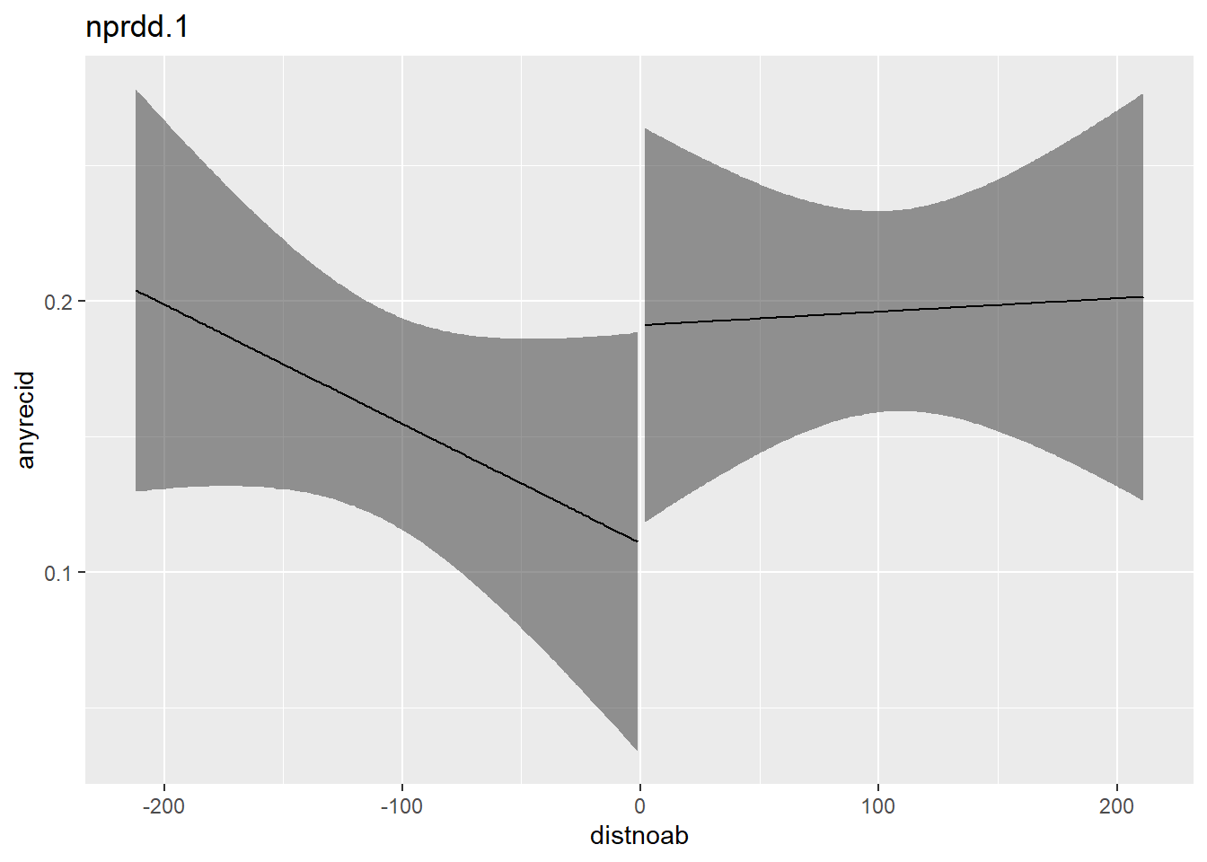
nprdd.1 <- lm(anyrecid ~ after * distnoab,
              data = flo,
              subset = (distnoab >= -212 & distnoab <= 212))
# summary(nprdd.1)
plot_with_ci(nprdd.1, lim_bandwith = T, lower = -212, upper = 212)
Note: If we call the summary() function on this model the estimated standard errors differ from those in Tuttle (2019) because Tuttle uses clustered standard errors that are clustered on distnoab. The use of standard errors that are clustered on the running variable are common in RD-designs but debatable (see Kolesar, M. und C. Rothe (2018), Inference in Regression Discontinuity Design with a discrete running variable, American Economic Review 108, S. 2277-2304)). An alternative could be robust standard errors.
To calculate clustered and robust standard errors the packages lmtest and sandwich can be used:
Tuttles clustered standard errors:
coeftest(nprdd.1, vcov = vcovCL, cluster = ~distnoab)
##
## t test of coefficients:
##
##                   Estimate  Std. Error t value  Pr(>|t|)
## (Intercept)     0.11062284  0.03281047  3.3716 0.0007839 ***
## after           0.08033841  0.04929772  1.6297 0.1035740
## distnoab       -0.00044003  0.00028580 -1.5396 0.1240489
## after:distnoab  0.00048961  0.00042046  1.1645 0.2445864
## ---
## Signif. codes:  0 '***' 0.001 '**' 0.01 '*' 0.05 '.' 0.1 ' ' 1
Robust standard errors:
coeftest(nprdd.1, vcov = vcovHC)
##
## t test of coefficients:
##
##                   Estimate  Std. Error t value  Pr(>|t|)
## (Intercept)     0.11062284  0.03341736  3.3103 0.0009743 ***
## after           0.08033841  0.05189668  1.5480 0.1220134
## distnoab       -0.00044003  0.00028184 -1.5613 0.1188639
## after:distnoab  0.00048961  0.00043667  1.1212 0.2625265
## ---
## Signif. codes:  0 '***' 0.001 '**' 0.01 '*' 0.05 '.' 0.1 ' ' 1
In a modelsummary table (note that the only difference is in the standard errors):
# Alternative: modelsummary()
models2 = list(
  "nprdd.1  classical se" = nprdd.1,
  "nprdd.1  clustered se" = nprdd.1,
  "nprdd.1  robust se" = nprdd.1
)
modelsummary(models2,
             stars = TRUE,
             fmt = 4, # 4 Nachkommastellen
             vcov = c("classical", ~distnoab, "HC1"))
| nprdd.1 classical se | nprdd.1 clustered se | nprdd.1 robust se | |
|---|---|---|---|
| (Intercept) | 0.1106** | 0.1106*** | 0.1106*** |
| (0.0396) | (0.0328) | (0.0333) | |
| after | 0.0803 | 0.0803 | 0.0803 |
| (0.0546) | (0.0493) | (0.0517) | |
| distnoab | -0.0004 | -0.0004 | -0.0004 |
| (0.0003) | (0.0003) | (0.0003) | |
| after × distnoab | 0.0005 | 0.0005 | 0.0005 |
| (0.0004) | (0.0004) | (0.0004) | |
| Num.Obs. | 791 | 791 | 791 |
| R2 | 0.005 | 0.005 | 0.005 |
| R2 Adj. | 0.001 | 0.001 | 0.001 |
| AIC | 731.5 | 731.5 | 731.5 |
| BIC | 754.8 | 754.8 | 754.8 |
| Log.Lik. | -360.741 | -360.741 | -360.741 |
| F | 1.288 | 1.641 | |
| RMSE | 0.38 | 0.38 | 0.38 |
| Std.Errors | IID | by: distnoab | HC1 |
| + p < 0.1, * p < 0.05, ** p < 0.01, *** p < 0.001 |
Table 3 from Snapping Back
In the following parts Table 3 from the Snapping Back paper will be recreated. Technically there is nothing new, the only change is in the used bandwith and type of recidivism as dependent variable.
Panel A: optimal bandwith
There exist several algorithms to calculate the optimal bandwith to get enough information to use on the one hand while not falling for non-linear longterm trends on the other hand. The values used here are simply those calculated by Tuttle.
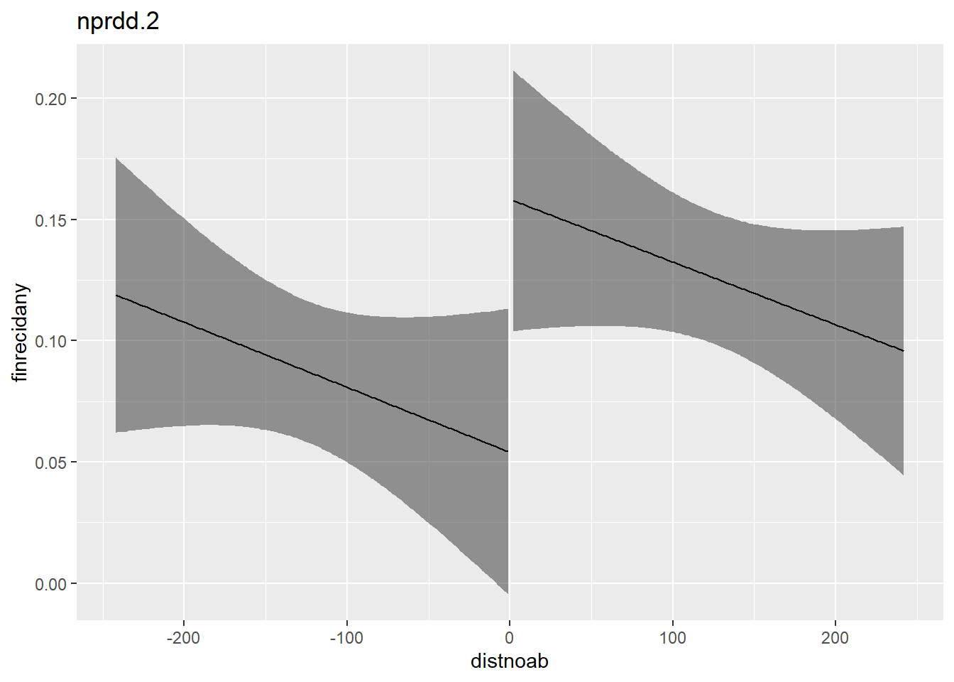
nprdd.2 <- lm(finrecidany ~ after * distnoab,
data = flo,
subset = (distnoab >= -242 & distnoab <= 242))
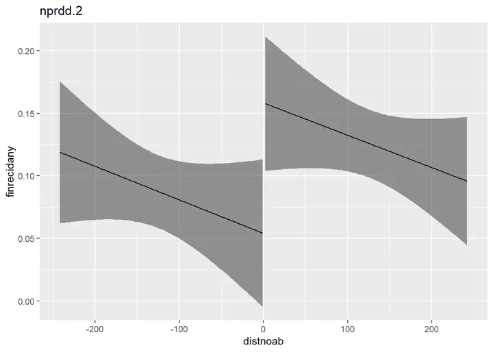
plot_with_ci(nprdd.2, response = finrecidany, lim_bandwith = T, lower = -242, upper = 242)
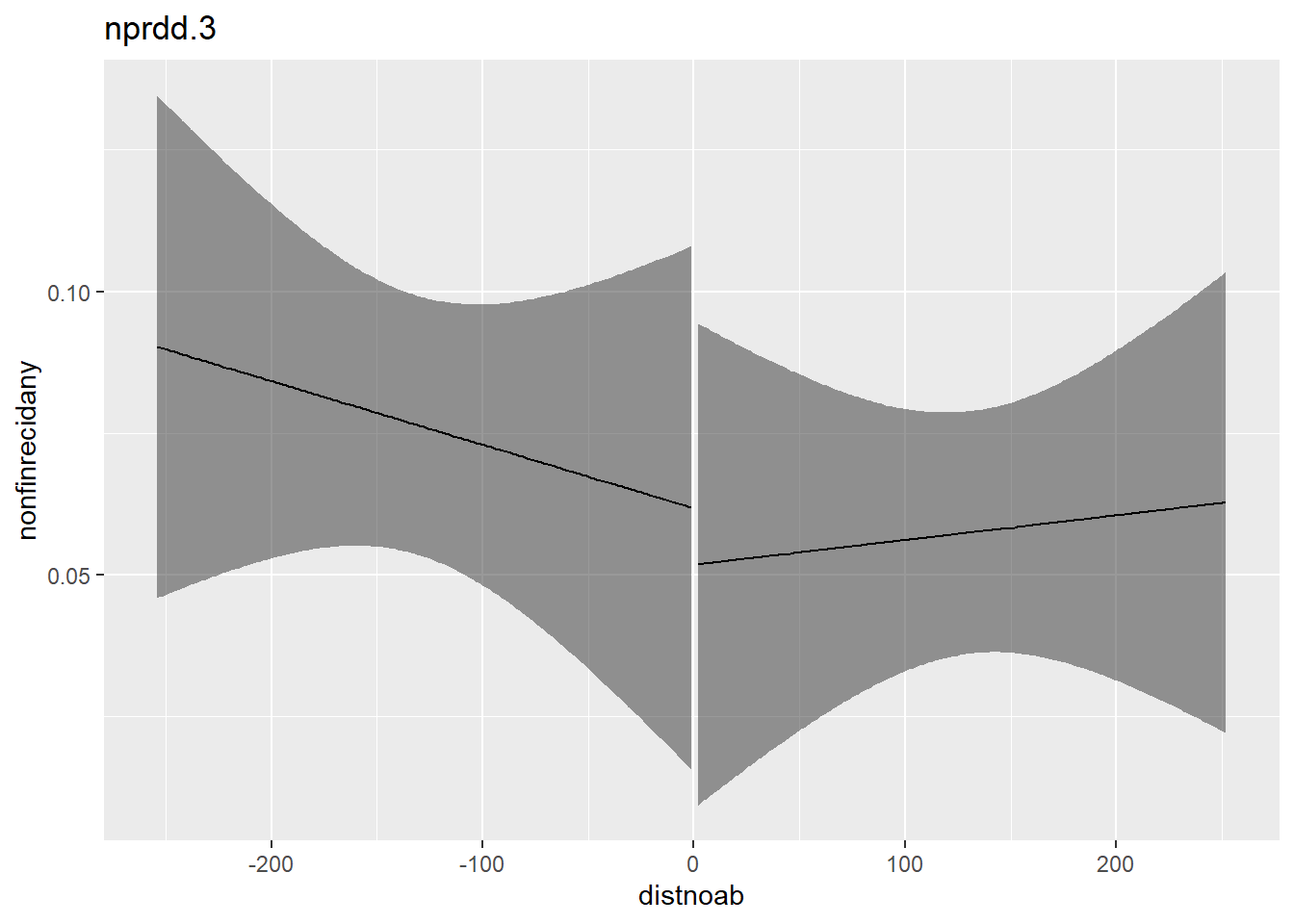
nprdd.3 <- lm(nonfinrecidany ~ after * distnoab,
              data = flo,
              subset = (distnoab >= -254 & distnoab <= 254))
plot_with_ci(nprdd.3, response = nonfinrecidany, lim_bandwith = T, lower = -254, upper = 254)
models3 = list(
  "nprdd.1 'Recidivism'" = nprdd.1,
  "nprdd.2 'Financially motivated recidivism'" = nprdd.2,
  "nprdd.3 'Non-financially motivated recidivism'" = nprdd.3
)
modelsummary(models3,
             stars = TRUE,
             fmt = 4,
             vcov =  ~distnoab)
| nprdd.1 'Recidivism' | nprdd.2 'Financially motivated recidivism' | nprdd.3 'Non-financially motivated recidivism' | |
|---|---|---|---|
| (Intercept) | 0.1106*** | 0.0540* | 0.0617** |
| (0.0328) | (0.0239) | (0.0214) | |
| after | 0.0803 | 0.1043** | -0.0100 |
| (0.0493) | (0.0398) | (0.0280) | |
| distnoab | -0.0004 | -0.0003 | -0.0001 |
| (0.0003) | (0.0002) | (0.0002) | |
| after × distnoab | 0.0005 | 0.0000 | 0.0002 |
| (0.0004) | (0.0003) | (0.0002) | |
| Num.Obs. | 791 | 936 | 980 |
| R2 | 0.005 | 0.007 | 0.002 |
| R2 Adj. | 0.001 | 0.004 | -0.001 |
| AIC | 731.5 | 468.4 | 62.9 |
| BIC | 754.8 | 492.6 | 87.4 |
| Log.Lik. | -360.741 | -229.178 | -26.473 |
| RMSE | 0.38 | 0.31 | 0.25 |
| Std.Errors | by: distnoab | by: distnoab | by: distnoab |
| + p < 0.1, * p < 0.05, ** p < 0.01, *** p < 0.001 |
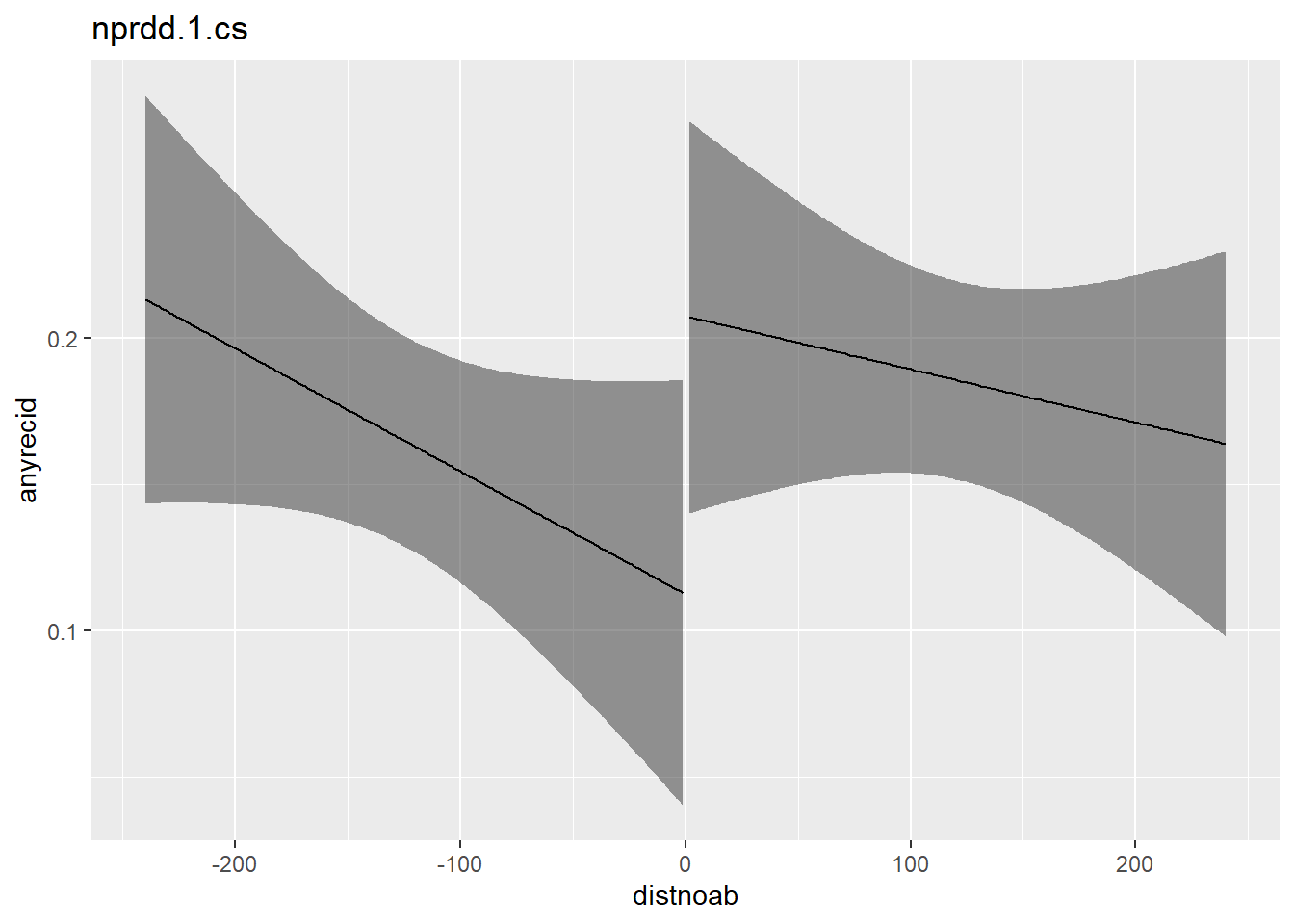
Panel B: consistent bandwith = 240 days
nprdd.1.cs <- lm(anyrecid ~ after * distnoab,
              data = flo,
              subset = (distnoab >= -240 & distnoab <= 240))
plot_with_ci(nprdd.1.cs, lim_bandwith = T, lower = -240, upper = 240)
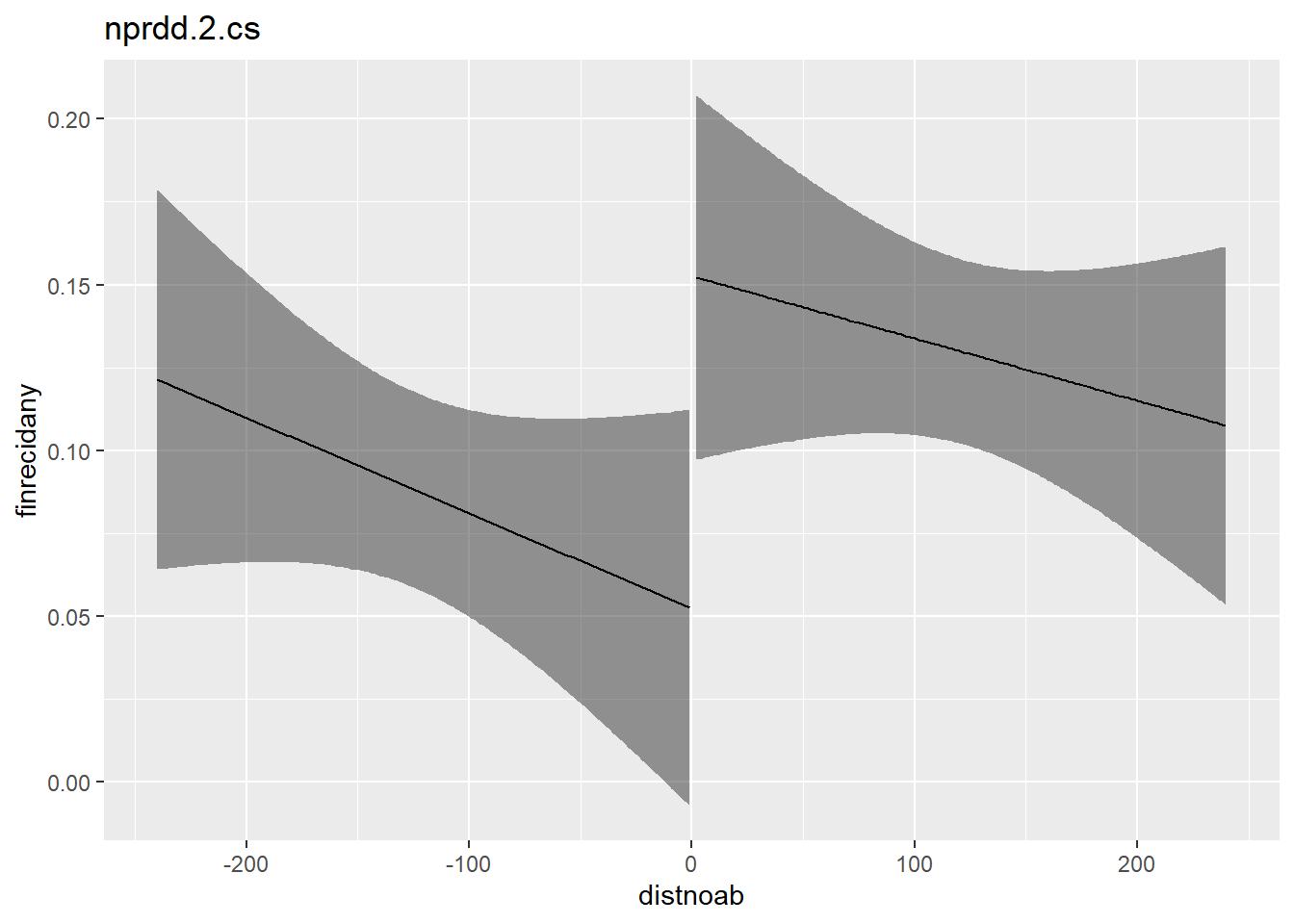
nprdd.2.cs <- lm(finrecidany ~ after * distnoab,
              data = flo,
              subset = (distnoab >= -240 & distnoab <= 240))
plot_with_ci(nprdd.2.cs, response = finrecidany, lim_bandwith = T, lower = -240, upper = 240)
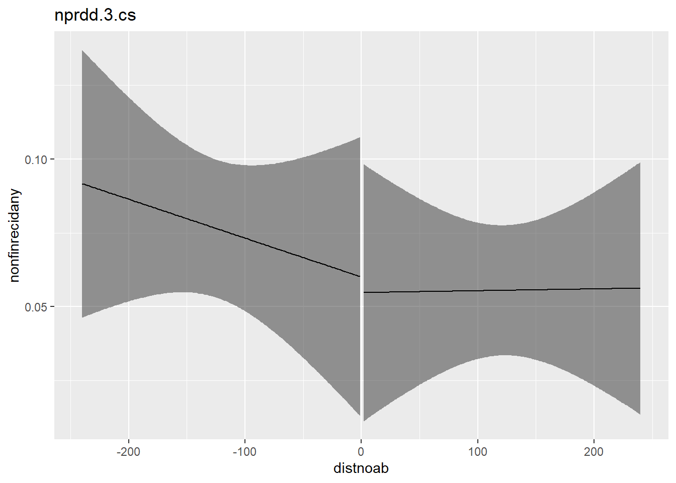
nprdd.3.cs <- lm(nonfinrecidany ~ after * distnoab,
              data = flo,
              subset = (distnoab >= -240 & distnoab <= 240))
plot_with_ci(nprdd.3.cs, response = nonfinrecidany, lim_bandwith = T, lower = -240, upper = 240)
models4 = list(
  "nprdd.1.cs 'Recidivism'" = nprdd.1.cs,
  "nprdd.2.cs 'Financially motivated recidivism'" = nprdd.2.cs,
  "nprdd.3.cs 'Non-financially motivated recidivism'" = nprdd.3.cs
)

modelsummary(models4,
             stars = TRUE,
             fmt = 4,
             vcov =  ~distnoab)
| nprdd.1.cs 'Recidivism' | nprdd.2.cs 'Financially motivated recidivism' | nprdd.3.cs 'Non-financially motivated recidivism' | |
|---|---|---|---|
| (Intercept) | 0.1124*** | 0.0523* | 0.0601** |
| (0.0323) | (0.0241) | (0.0221) | |
| after | 0.0950* | 0.1003* | -0.0053 |
| (0.0467) | (0.0404) | (0.0286) | |
| distnoab | -0.0004 | -0.0003 | -0.0001 |
| (0.0003) | (0.0002) | (0.0002) | |
| after × distnoab | 0.0002 | 0.0001 | 0.0001 |
| (0.0004) | (0.0003) | (0.0002) | |
| Num.Obs. | 918 | 918 | 918 |
| R2 | 0.004 | 0.007 | 0.002 |
| R2 Adj. | 0.001 | 0.004 | -0.001 |
| AIC | 836.3 | 475.3 | 46.7 |
| BIC | 860.4 | 499.4 | 70.8 |
| Log.Lik. | -413.144 | -232.668 | -18.362 |
| RMSE | 0.38 | 0.31 | 0.25 |
| Std.Errors | by: distnoab | by: distnoab | by: distnoab |
| + p < 0.1, * p < 0.05, ** p < 0.01, *** p < 0.001 |
Calculating optimal bandwidth
The optimal bandwith can generally be calculated with the function IKbandwith from the rdd package. The function does not work on the specific data here though, for unknown reasons.
library(rdd)
## Lade nötiges Paket: Formula
IKbandwidth(X = flo$distnoab, Y = flo$anyrecid, cutpoint = 0, verbose = T, kernel = "rectangular")
## Error in if (sum(left) == 0 | sum(right) == 0) stop("Insufficient data in the calculated bandwidth."): Fehlender Wert, wo TRUE/FALSE nötig ist