Income inequality and demand for redistribution in Austria
The Corona pandemic reinforced the trend of the rich getting richer and the poor getting poorer. According to Oxfam the “Richest 1% bag nearly twice as much wealth as the rest of the world put together over the past two years” (Oxfam, 2003) and “ten richest men double their fortunes in pandemic while incomes of 99 percent of humanity fall” (Oxfam 2022). At least in theory and democratic countries there seems to be an easy solution for those not belonging to the top percent: voting for more redistribution. Yet we still see concentration of wealth in democracies. There could be several reasons for this. The first one being that the people don’t know about the degree of inequality.
Another one would be that they do know about the inequality but don’t think that inequality is a bad thing, e.g., because they consider the respective wealth of the richer folks was justly earned. In both cases the inequality would not lead to more demand for redistribution. If there actually is a demand for redistribution there are still ways that prevent more redistribution from happening. People not trusting the political system and therefore not voting for more redistribution, even though they support it, for example, or people might vote for parties that advertise themselves as being for more redistribution but when in power the parties don’t stay true to their promises.
In this article I will firstly look into the relation of inequality and demand for redistribution in Austria. The theoretical point of departure for this analysis will be the Meltzer-Richard-Model. On ground of that model the hypothesis that more income inequality has a positive effect on demand for redistribution will be tested as well as the hypothesis that income has a negative effect on demand for redistribution. To test these hypothesis a multilevel model on European-Social-Survey data will be applied. There was no evidence found for a significant effect of income inequality on demand for redistribution in Austria while evidence for the negative effect of income on demand for redistribution was found. Secondly, I will briefly look into whether different voting behaviour across income deciles can shed light on why there is not more political demand for redistribution, finding that those who would profit from more redistribution are also those less likely to vote.
Literature Review
The Meltzer-Richard model
In their 1981 paper A Rational Theory of the Size of Government Allan H. Meltzer and Scoot F. Richard seek an explanation for the increased share of income allocated by government. They note that “government spending and taxes have grown relative to output in most countries with elected governments for the past 30 years or longer” (Meltzer & Richard, 1981, p. 924) and that this growth “appears to be independent of budget and tax systems, federal or national governments, the size of the bureaucracy and other frequently mentioned institutional arrangements” (ibid.). The explanation of said development of increased relative government spending Meltzer and Richard provide is based on voter demand for redistribution. Their model assumes that the government is only collecting taxes and redistributing them again. Hence the government provides no services or public goods in this model.
Furthermore, the tax rate is assumed to be linear, real budget is assumed to be balanced and voters are assumed to be fully informed. Under these assumptions they provide an argument for the size of government being determined by the welfare-maximizing choice of a decisive individual. Their “hypothesis implies that the size of government depends on the relation of mean income to the income of the decisive voter" (ibid., p. 916). Under reference of Roberts (1977) they argue that “with universal suffrage the voter with median income is decisive, and the higher one’s income the lower the preferred tax rate” (Meltzer & Richard, 1981, p. 921). They further argue that “the decisive voter chooses the tax share” (ibid., p. 924) and voters below the income of the decisive voter prefer a higher tax share while those with a higher income than that of the decisive voter prefer a lower tax share.
The basic argument, even though it “explains too much” (ibid., p. 916) according to Meltzer and Richard is that the mean income is larger than the median income in industrialized countries and the mean voter therefore profits from redistribution, as long as the mean income is still above the median income. Since according to this too simple approach the mean income would eventually equal the median income Meltzer and Richard take into account considerations of the decisive voter regarding the “disincentive effects created by redistribution (e.g. lower labor supply), so that redistribution will not be perfect” (Finseraas, 2009, p. 97). Meltzer and Richard find evidence for their model in the increase of tax share which followed the increased numbers of voters with relatively low income.
Other models and studies
Iversen (2005) proposes another model that differs from the MRM “because it emphasizes the distribution of risk and skills for level of redistribution, rather than the distribution of income” (Finseraas, 2009, p. 97) but also supports the same hypothesis that inequality is positively correlated with demand for redistribution. A more complex model by Moene and Wallerstein (2001, 2003) is presented, in which “total spending has a V-shaped association with equality” (Finseraas 2009, p. 98). It is also pointed out though “that if an increase in inequality is due to an increase in average income rather than a fall in median income […], then the demand for welfare spending will increase with inequality even in the Moene and Wallerstein model” (ibid.) and that indeed the increase in inequality is largely due to the rise in top incomes (vgl. ibid; Scheve & Stasavage, 2007, p. 6). Empirical studies have found mixed evidences, Aalberg (2003) finds support for the assumed inequality-redistributiondemand relation, while Roller (1995) finds positive correlations in some times but not in others and Bowles and Gintis (2000) even find a negative correlation while Lübker (2007) only finds an insignificant effect. Finseraas own finding is that “inequality is positively related with demand for redistribution” (Finseraas, 2009, p. 1). Another study has been conducted by Dallinger, who proposes a model of “contingent support for redistribution […], where culturally influenced definitions are embedded in economic processes” (2010, p. 1). Further studies that go beyond purely economic factors have for example been conducted by Burgoon who found that “exposure to higher foreign-born percentages tends to diminish support for redistribution and social protection” (Burgoon, 2014, p. 366) and Stegmüller et al (2012) who found that religious people are more likely to oppose redistribution by the state. Dimick and associates (2016) analysed whether other regarding preferences effect demand for redistribution with the result that data for the United States support the hypothesis that rich people, while preferring less redistribution than poor people, are more responsive to changes in inequality than poor people. Cleiton Robert da Fonseca Silva and Erik Alencar de Figueiredo looked into social mobility and the demand for income redistribution in Latin America (2013), with the result, that demand for redistribution in Latin America is driven by educational level (contrary to the MRM demand increases with educational level though), self-interest and perceived inequality in opportunities. Past social downward mobility was found to have a significant positive influence on demand for redistribution while they found no evidence for the thesis that the prospect of upwards mobility influences demand for redistribution. The prospect of social upwards mobility thesis has also been tested by Roland Benabou and Efe A. OK (2001) using data from the USA, they could not find a significant effect either though.
Further theoretical considerations
Hypothesis to test
The Meltzer-Richard model offers a choice of hypothesis to test. In this chapter the hypothesis that will actually be tested and their relationship to the Meltzer-Richard model will be presented. The first Hypothesis is
H1: In Austria, years with a higher ratio of mean income to median income also have a higher demand for redistribution.
This hypothesis is based on two of Meltzer and Richards own hypothesis, namely “that the size of government depends on the relation of mean income to the income of the decisive voter” (Meltzer & Richards, 1981, p. 916) and that “with universal suffrage the voter with median income is decisive” (ibid., p. 921). Since only the development in Austria will be analysed in this study it seems fair to assume universal suffrage and therefore work with the median income as the income of the decisive voter, which makes the size of government depend on the relation of mean income to median income. Meltzer and Richard’s measure is not demand for redistribution as in the presented hypothesis H1, but size of government. Since size of government is just the amount of redistribution in their model and said amount only depends on the (median) voter’s preference, demand for redistribution seems to be the decisive factor for the size of government and can therefore be used in the hypothesis, which leads us to the demand for redistribution being dependent on the relation of mean income to median income.
This approach of using demand for redistribution instead of size of government has been applied before as well. Finseraas for example explicitly distinguishes two steps in Meltzer and Richard’s model, the first one being that inequality determines demand for redistribution and the second being that said demand actually determines the level of redistribution (2009, p. 97). Under reference of Lübker (2007) he points out that “the first step of the argument – inequality determines the demand for redistribution – is simply taken for granted” and sets out to test this “first chain of the argument” (Finseraas, 2009, p. 97). I will follow his example in this article. It is fair to assume that mean and median income refer to country mean and median, which was the last missing piece in deriving H1.
The second hypothesis H2 is derived directly from “the higher one’s income the lower the preferred tax rate” (Meltzer & Richard 1981, 921) by using demand for redistribution instead of preferred tax rate:
H2: The higher the income of an individual the lower the demand for redistribution of the individual.
Therefore, we have one hypothesis to test on the individual level and one hypothesis on the year level.
Measuring inequality
The MRM makes it quite clear that the ratio of mean income to median income is the decisive factor when it comes to demand for redistribution. However, the underlying question can be asked in a more general way, namely whether inequality leads to a higher demand for redistribution. To answer that question on has to define a way to measure inequality. Even if we restrict inequality to income inequality, there are still several ways to measure it. The most prominent measure is probably the GINI coefficient, which is for example used by Finseraas (2009) to test whether inequality is positively associated with demand for redistribution. As pointed out several times before, the measure that comes closest to the MRM is the mean-median-ratio.
But does it make a difference whether we use the GINI-coefficient or the mean-median-ratio? The GINI-coefficient basically measures whether everyone gets an equal slice of the income cake, in which case the coefficient would be 0 with higher values indicating more inequality and the coefficient being 1 if one person has all the income. That makes the coefficient sensitive to equal increases of income for every individual though, since those reduce the relative difference in slice sizes. Suppose a former income poor country finds large amounts of oil and decides to redistribute the accompanying profits. If everyone has an income bonus of 1 million dollars through that redistribution it does not matter that much whether they made 1000USD or 3000USD before, they pretty much have the same income now. And the GINI coefficient will reflect that.
If the income distribution before the oil money was normally distributed, I.e., median and mean were equal, the distribution will still be normally distributed and mean and median will therefore still be equal after the redistribution though. Consequently, the mean-median-ratio would not change in this scenario either, contrary to the GINI-coefficient. It can therefore make a difference which of the two measures one chooses, even though it has to be said that income distributions are typically not normally distributed and changes in income will usually not be equal across individuals either. Even so, they are different measures and to make things worse not the only two to choose from, Dimick and associates for example identify inequality with the social welfare function (2016, p. 390f) in their aforementioned model. So how to decide on one measure? Blesch and associates suggest “a bottomup and data-driven approach that draws on the shape of actual income distributions” (2022, p. 2).
Against their advice I will simply use the GINI coefficient and see whether the results are robust to using the mean-median-ratio, ignoring possible other measures.
Data and Method
In this chapter the used data and methods will be presented. The data used consists of round one to nine of the European Social Survey, minus round six, due to not including Austria.
Dependent Variable
Following previous studies preference for redistribution will be measured through the question ‘the government should take measures to reduce differences in income levels’. Respondents can express their agreement in five categories ranging from ‘agree strongly’ to ‘disagree strongly’. The distribution of the pooled sample is given in figure 1 while figure 2 visualizes the distribution per country. In the sampled data the vast majority of the 17187 respondents who answered the question agrees (42%) or agrees strongly (30%) with the statement “Government should reduce differences in income levels”, while 15% were indifferent and only few disagreeing (9%) or disagreeing strongly (4%). Further summary statistics regarding the demand for redistribution as well as other variables and their correlations can be found in Appendix A.
Figure 1 Demand for income redistribution across all years, coloured by household income decile
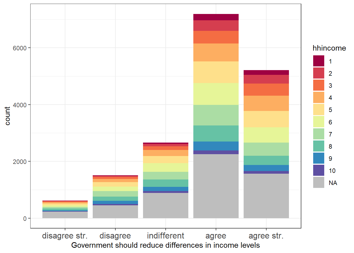
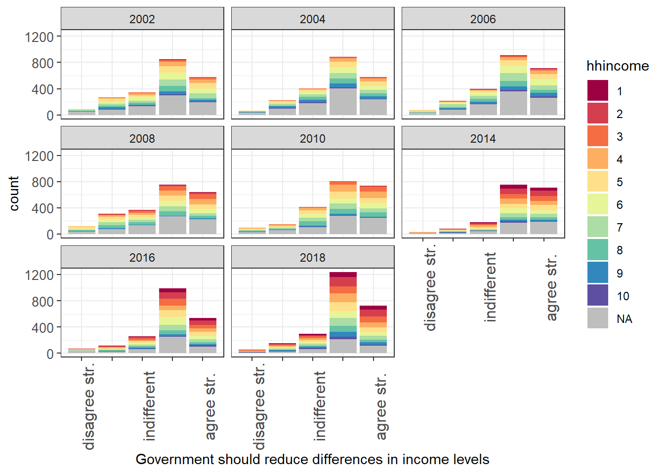
Figure 2 Demand for redistribution per year, coloured by household income decile.
Independent Variables
The Meltzer-Richard-model is quite parsimonious when it comes to explanatory variables: All that is needed is basically the income of individuals. From those the mean and median income can be calculated. Demand for redistribution of an individual is then given through the relations between the individual’s income and the mean and median income. The mean-median-ratio is calculated by the mean and median income before social transfers (pensions included in social transfers) of the respective countries, with data taken from Eurostat.
The mean-median-ratio ranges from 1.087 to 1.128 with a mean of 1.106 and a standard derivation of 0.016. While the GINI-coefficient ranges from 25.3 to28.3, with a mean of 26.916 and a standard derivation of 1.011. The household income in the ESS is given in deciles of the actual household range in the given country. The household income has been given by 68% of respondents.
As control variables such variables have been chosen that might influence expected income and are available for each round. Those variables are only gender and age in this study. The argument for using gender is that women are thought to be disadvantaged in the labor market and aware of that. So, other things being equal, women have to assume that they are more likely to be in need of redistribution at one point than their male counterparts. Which gives them an incentive for supporting more redistribution. A similar point can be made for age. Age will be included in quadratic form, since support for redistribution is expected to sink when earning more money as one grows older but also grow again when the retirement age is (soon to be) reached.
Model
To analyse the data the following multilevel model will be applied with random slopes and random intercepts for household income and gender:
$$` \begin{aligned} \operatorname{gincdif}_{i} &\sim N \left(\mu, \sigma^2 \right) \\ \mu &=\alpha_{j[i],k[i]} + \beta_{1j[i]}(\operatorname{hhincome})\ + \\ &\quad \beta_{2}(\operatorname{hhmembers}) + \beta_{3k[i]}(\operatorname{gender}_{\operatorname{female}})\ + \\ &\quad \beta_{4}(\operatorname{age}) + \beta_{5}(\operatorname{age\ *\ age}) \\ \left( \begin{array}{c} \begin{aligned} &\alpha_{j} \\ &\beta_{1j} \end{aligned} \end{array} \right) &\sim N \left( \left( \begin{array}{c} \begin{aligned} &\gamma_{0}^{\alpha} + \gamma_{1}^{\alpha}(\operatorname{GINI}) \\ &\mu_{\beta_{1j}} \end{aligned} \end{array} \right) , \left( \begin{array}{cc} \sigma^2_{\alpha_{j}} & \rho_{\alpha_{j}\beta_{1j}} \\ \rho_{\beta_{1j}\alpha_{j}} & \sigma^2_{\beta_{1j}} \end{array} \right) \right) \\ &\text{for year j = 1,} \dots \text{,J} \\ \left( \begin{array}{c} \begin{aligned} &\alpha_{k} \\ &\beta_{3k} \end{aligned} \end{array} \right) &\sim N \left( \left( \begin{array}{c} \begin{aligned} &\mu_{\alpha_{k}} \\ &\mu_{\beta_{3k}} \end{aligned} \end{array} \right) , \left( \begin{array}{cc} \sigma^2_{\alpha_{k}} & \rho_{\alpha_{k}\beta_{3k}} \\ \rho_{\beta_{3k}\alpha_{k}} & \sigma^2_{\beta_{3k}} \end{array} \right) \right) \\ &\text{for year j = 1,} \dots \text{,J} \\ \end{aligned}$$`Furthermore, the same model will be applied with mean-median-ratio instead of the GINI-coefficient to make results more robust. Another model that will be used with the same intention is a linear regression model with clustered standard errors and the GINI-coefficient as inequality measure.
Results
As we can see in Table 1 there is no significant effect of income inequality on demand for redistribution. This result is robust to using the mean-median-ratio instead of the GINI-coefficient for using income inequality as well as using the different modelling approach with clustered standard errors. While the estimate of the GINI coefficient differs by direction and roughly factor 10 between the clustered standard error model and multilevel model, effects in both models are substantially and statistically insignificant. If not stated otherwise the multilevel model using the GINI-coefficient is used in the following discussion.
The effect of household income is statistically significant, with the direction as expected: higher income is associated with lower demand for redistribution. The effect size is visualized in figure 3. The expected direction of effect holds for every year, while the slopes and intercepts differ. With the exceptions of 2008 and 2010 the mean of demand for redistribution per household income decile falls into the agree range across all deciles. In 2008 the mean is closer to ‘indifferent’ than to ‘agree’ from the seventh decile on, in year 2010 the last decile is.
Table 1 Regression results
| Multilevel GINI | Multilevel Mean/Median | Clustered se | |
|---|---|---|---|
| Intercept | 0.8882 | -0.9215 | 1.5611 |
| (0.7524) | (3.3363) | (1.2013) | |
| gini | 0.0029 | -0.0239 | |
| (0.0274) | (0.0415) | ||
| household income | -0.0582*** | -0.0584*** | -0.0608*** |
| (0.0141) | (0.0142) | (0.0122) | |
| household members | -0.0068 | -0.0073 | -0.0037 |
| (0.0089) | (0.0089) | (0.0097) | |
| genderFemale | 0.1995*** | 0.2006*** | 0.1978*** |
| (0.0402) | (0.0342) | (0.0383) | |
| age | 0.0104*** | 0.0104*** | 0.0123+ |
| (0.0030) | (0.0030) | (0.0070) | |
| age*age | -0.0001*** | -0.0001*** | -0.0001* |
| (0.0000) | (0.0000) | (0.0001) | |
| mean/median | 1.7095 | ||
| (3.0150) | |||
| SD (Intercept year) | 0.1411 | 0.0000 | |
| 0.1411 | 0.0995 | ||
| 0.1707 | 0.0000 | ||
| 0.1707 | 0.0995 | ||
| SD (household income year) | 0.0346 | 0.0349 | |
| SD (genderFemale year) | 0.0922 | 0.0732 | |
| Cor(Intercept~household income year | -1.0000 | -0.1274 | |
| Cor(Intercept~genderFemale year | -1.0000 | ||
| SD (Observations) | 1.0137 | 1.0139 | |
| Num.Obs. | 10382 | 10382 | 10382 |
| R2 Adj. | 0.028 | ||
| R2 Marg. | 0.028 | 0.029 | |
| + p < 0.1, * p < 0.05, ** p < 0.01, *** p < 0.001 |
Figure 3 Effect of household income on demand for redistribution per year with mean effect over all
years in blue and bold.

The effect of gender is statistically significant, with females demanding more redistribution on average. The effect across all years can be seen in figure 4. In most years the mean demand for redistribution falls into the ‘agree’ category for both males and females, with a similar difference between males and females across years and with the more recent years tending to have a higher mean demand for redistribution. Year 2008 is the exception with males being closer to indifferent than to agreeing and a noticeably higher difference in agreement to redistribution between males and females.
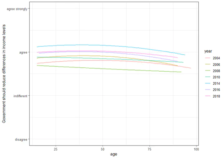
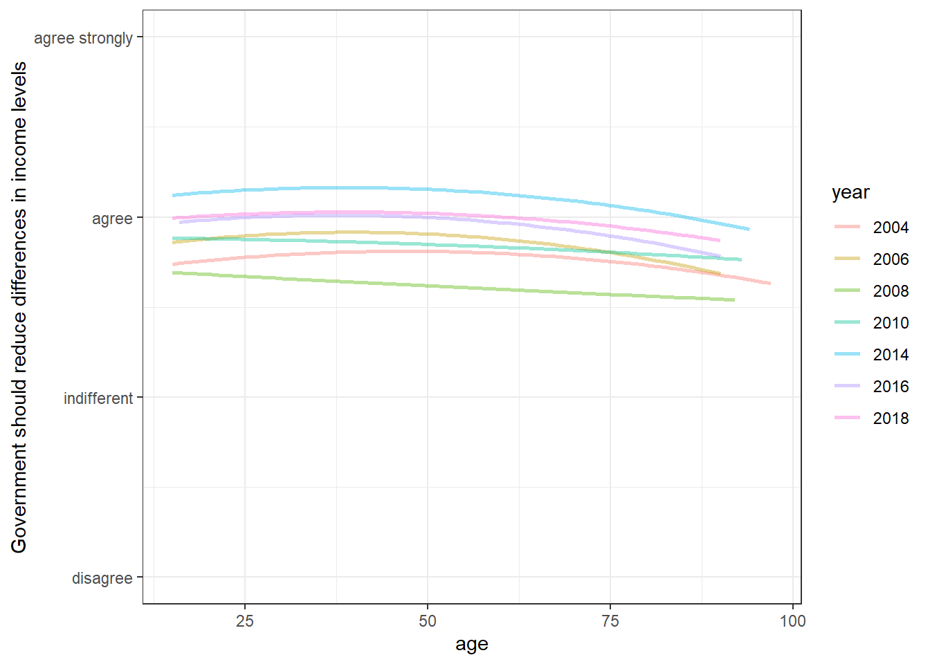
The effect of age is statistically significant but not quite as expected: Instead of higher agreement when one is likely not the one paying for it, i.e., when one is young and old, the curve is reversed, with the lowest agreement under the youngest and oldest, except for 2008 and 2010. Across all ages and all years the mean is agreeing with more redistribution though as seen in Figure 5.
Given the low R^2 values and the fact that the income inequality is not statistically significant at all, we can conclude that focusing on income inequality and (household-) income in accordance with the MRM does not offer much power to explain demand for redistribution in Austria in the examined years. While the demand for redistribution decreases with income most people agree with more redistribution even in the highest income decile across most years.
Figure 4 Effect of gender on demand for redistribution per year.
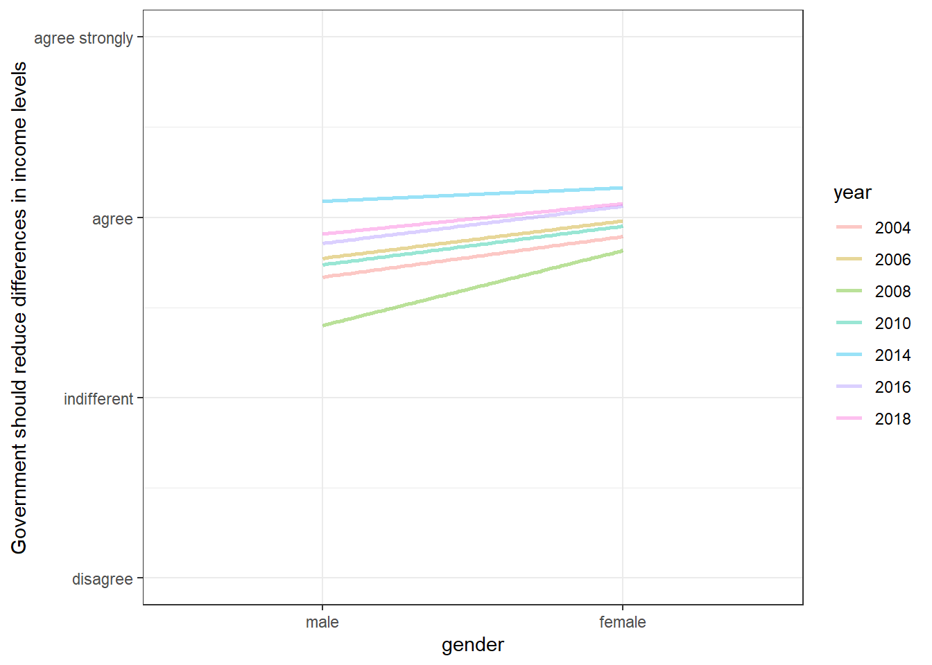
Figure 5 Effect of age on demand for redistribution per year.
Income and voting
There were several points that could prevent redistribution: People not wanting more redistribution, people wanting redistribution but not voting for more redistribution and people voting for more redistribution but political parties not acting accordingly. The first point does not seem to be given if we look at the previous part’s results. So, let’s look into the voting behaviour.
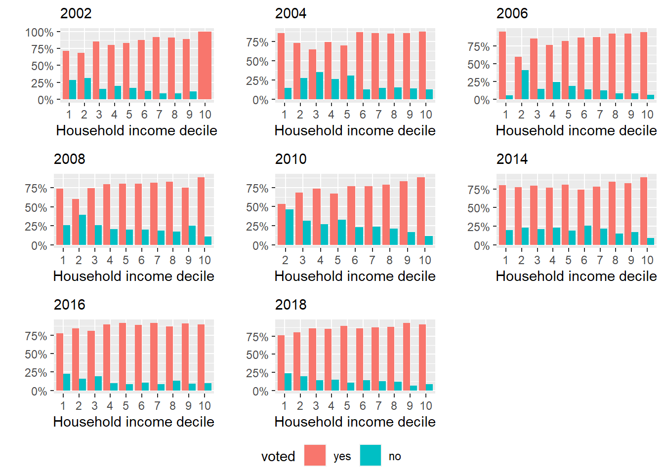
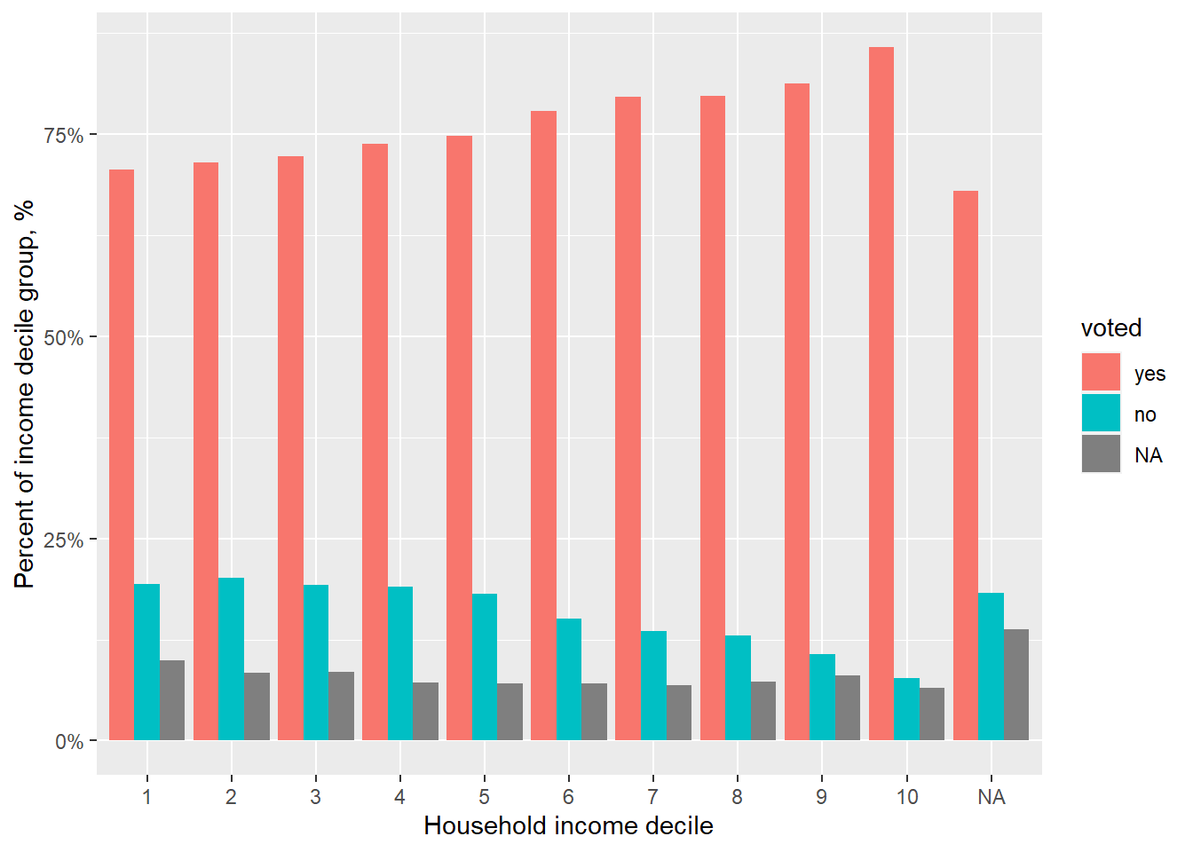
Assuming that those in lower income deciles are those that would benefit from more income redistribution and that there is higher demand for redistribution in those deciles, a lower voter turnout in those deciles could possibly lead to less political demand for redistribution. Figure 6 shows that across all years there is indeed a difference in voter turnout between income deciles. While in the lowest decile 71% of the respondents voted and 19% did not vote and 10% didn’t answer or were not allowed to vote, the number of voters continuously increases across the deciles to 85% in the tenth decile, with the percent of non-voters with 8% being less than half the number of non-voters in the first decile. Appendix B visualizes the relation for all years separately.
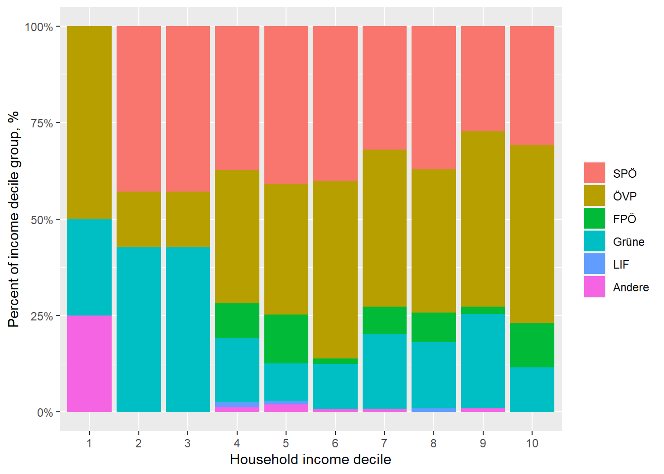
To see whether those who do vote differ in who they vote for between the different income decile groups, we are somewhat limited by the data in the ESS, since for a lot of rounds this data is not provided. As an exemplification we will have one look at the second ESS round, where the data is provided. The results are visualized in figure 7. This figure illustrates two points: First, there are very few respondents in the first and second income deciles and still relatively few respondents in the third and tenth income decile. This is quite a problem for the analysis and one that is not limited to the voting question.
Figure 6 Share of people who voted per household income decile across all years. People not eligible to vote were counted as NA.
Second, in those income deciles where we do have data, there is not a lot of difference in the voting pattern. There is a trend of decreasing support for SPÖ with increasing household income and the reverse trend if we look at support of ÖVP. Continuing this analyses by looking into how the political program of the respective parties looks like and what measures they implemented (or opposed) to increase redistribution would be too much for this article so those questions will be left open. It seems like a fair guess that the SPÖ is more likely to be in favour of redistribution than the ÖVP though. Accepting that, the trend of increased support for ÖVP and that the members of higher income deciles are also the ones most likely to vote one might have explained a (minor) part of why there is not more redistribution in Austria.
Figure 7 Number of votes per party and income decile.
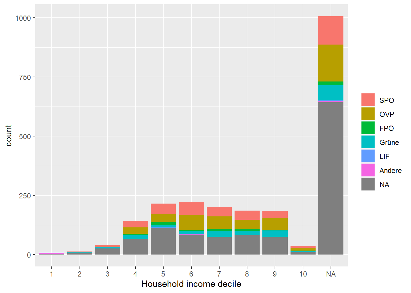
Figure 8 share of votes per income decile, missings excluded.
Conclusion and limitations
The question starting this article was why there is not more redistribution happening in Austria, given the social inequality and democratic system. We identified several possible reasons: There could simply be no demand for more redistribution, there could be demand for more redistribution but that demand does not find it’s way into the political system and there could be demand that is carried into the political system by voters but not acted on by politicians. The focus of this article was mainly on the first possible reason, looking into whether social inequality leads to an increased demand for redistribution.
On ground of the Meltzer-Richard-Model the hypothesis to test was that social inequality does indeed increase demand for redistribution. To test this hypothesis a multilevel model was applied to several rounds of the ESS. The model suggests that there is no significant effect of social inequality on demand for redistribution, while there is a significant effect of household income, gender and age. We also found that in most years the vast majority of respondents are in favour of more redistribution through all income deciles, gender and ages. Limitations of this approach are the low number of years (and accompanying inequality measures) that went into the model, due to there not being more rounds of the ESS available as well as missing data when it comes to income deciles. There were also some inconsistencies through the rounds of the ESS regarding the items. Educational level for example was measured but in some rounds the scale that was used could not be transferred to the EISCED scale used in other rounds. Including the educational level showed a significant effect for those rounds where it was used. Using educational level of the respondent combined with the educational level of the parents could also be used to measure social mobility and its effect on demand for redistribution. So, creating a common scale across all rounds would be one approach to improve this article. Another thing that might be worth to look into is wealth inequality instead of income inequality as well as individual income instead of household income.
Looking at the voting behaviour across income deciles we found that the lowest income deciles, who would benefit the most from redistribution and also have the highest mean demand for redistribution, are also the decilesleast likely to vote and vice versa, a first hint at why there is not more redistribution. Digging deeper into the voting behaviour we faced the problem of missing data on who the respondents voted for in many rounds of the ESS. Furthermore, there are only very few observations in the two lower income deciles as well as in the highest income decile. In the income deciles where we have more observations, we found some rather minor difference in the parties voted for. Therefore, we have some minor evidence of the income decile (and therefore of being a profiteer of more redistribution) having an effect on the party voted for.
References
Aalberg, T. 2003. Achieving Justice: Comparative Public Opinion on Income Distribution. Leiden: Brill.
Benabou, Roland and Efe A. Ok. “Social Mobility And The Demand For Redistribution: The Poum Hypothesis,” Quarterly Journal of Economics, 2001, v116(2,May), 447-487.
Blesch, K., Hauser, O. P., & Jachimowicz, J. M. (2022). Measuring inequality beyond the Gini coefficient may clarify conflicting findings. Nature Human Behaviour, 1–12. https://doi.org/10.1038/s41562-022-01430-7
Bowles, S. & Gintis, H. 2000. Reciprocity, Self-interest and the Welfare State. Nordic Journal of Political Economy 30, 33–53.
Burgoon, B. 2014. Immigration, Integration, and Support for Redistribution in Europe. World Politics, 66(3), 365-405.
Dalliner, U. 2010. Public support for redistribution: what explains cross-national differences? , Journal of European Social Policy 20, 333-349.
Dimick, M., Rueada, D., Stegmueller, D. 2016. The Altruistic Rich? Inequality and Other-Regarding Preferences for Redistribution. Quarterly Journal of Political Science, 11, 385-439.
Finseraas, H. 2009. Income Inequality and Demand for Redistribution: A Multilevel Analysis of European Public Opinion. Scandinavian Political Studies 32, 94-119.
Iversen, T. 2005. Capitalism, Democracy and Welfare. Cambridge: Cambridge University Press.
Lübker, M. 2007. Inequality and the Demand for Redistribution: Are the Assumptions of the New Growth Theory Valid? Socio-Economic Review 5, 117–48.
Meltzer, A. H. & Richard, S. F. 1981. A Rational Theory of the Size of Government. Journal of Political Economy 89, 914–27.
Moene, K. O. & Wallerstein, M. 2001. Inequality, Social Insurance and Redistribution. American Political Science Review 95, 859–74.
Moene, K. O. & Wallerstein, M. 2003. Earnings Inequality and Welfare Spending: A Disaggregated Analysis. World Politics 55, 485–516.
Oxfam, 2022. Ten richest men double their fortunes in pandemic while incomes of 99 percent of humanity fall. Press release publish 17th January 2002. Online: https://www.oxfam.org/en/press-releases/ten-richest-men-double-their-fortunes-pandemicwhile-incomes-99-percent-humanity (last visited 18.02.2023).
Oxfam, 2023. Richest 1% bag nearly twice as much wealth as the rest of the world put together over the past two years. Press release published 16th January 2023. Online: https://www.oxfam.org/en/press-releases/richest-1-bag-nearly-twice-much-wealth-restworld-put-together-over-past-two-years (last visited 18.02.2023).
Roberts, Kevin W. S. 1977. Voting over Income Tax Schedules. J. Public Econ. 8, 329-40.
Roller, E. 1995. The Welfare State: The Equality Dimension, in Borre, O. & Scarbrough, E., eds, The Scope of Government. Oxford: Oxford University Press.
Scheve, K. & Stasavage, D. 2007. Political Institutions, Partisanship and Inequality in the Long Run. Paper presented at the Comparative Politics of Inequality and Redistribution Seminar, Princeton, NJ, 11–12 May.
Silva, Cleiton & Figueiredo, Erik. (2013). Social mobility and the demand for the redistribution of income in Latin America. CEPAL review. 69-84.
Stegmueller, D., Scheepers, P., Roßteutscher, S., de Jong, D. 2012. Support for Redistribution in Western Europe: Assessing the role of religion, European Sociological Review, Volume 28, Issue 4, 482–497
Appendix A
| Unique (#) | Missing (%) | Mean | SD | Min | Median | Max | ||
|---|---|---|---|---|---|---|---|---|
| demand for redistribution | 6 | 3 | 0.9 | 1.1 | -2.0 | 1.0 | 2.0 | |
| GINI | 8 | 13 | 26.9 | 1.0 | 25.3 | 27.2 | 28.3 | |
| mean-median-ratio | 8 | 13 | 1.1 | 0.0 | 1.1 | 1.1 | 1.1 | |
| household income | 11 | 32 | 5.5 | 2.2 | 1.0 | 6.0 | 10.0 | |
| number of household members | 12 | 0 | 2.5 | 1.4 | 1.0 | 2.0 | 12.0 | |
| gender | 2 | 0 | 1.5 | 0.5 | 1.0 | 2.0 | 2.0 |
| demand for redistribution | GINI | mean-median-ratio | household income | number of household members | gender | |
|---|---|---|---|---|---|---|
| demand for redistribution | 1 | . | . | . | . | . |
| GINI | .02 | 1 | . | . | . | . |
| mean-median-ratio | -.03 | .67 | 1 | . | . | . |
| household income | -.13 | -.16 | .02 | 1 | . | . |
| number of household members | -.04 | -.14 | -.03 | .44 | 1 | . |
| gender | .09 | .00 | -.01 | -.06 | .01 | 1 |
Apendix B